7. Indexing and transposing a table
In this lecture we demonstrate:
- how indexing a table provides flexible access to the elements of the table;
- how to compute accross rows and columns of the table; and
- how to transpose a table.
7.1. Indexing
We have seen that working with columns of a DataFrame is very easy because colums have names. It would be as easy to work with rows of a DataFrame if we had a way to name the rows somehow. The process that does precisely that is called the indexing of a table.
To index a table we first have to identify a column (the indexing column or the index) such that each row in uniquely determined by the value in the indexing column. For example, in the following table
| Name | Sex | Age (yrs) | Weight (kg) | Height (cm) |
|---|---|---|---|---|
| Anne | f | 13 | 46 | 160 |
| Ben | m | 14 | 52 | 165 |
| Colin | m | 13 | 47 | 157 |
| Diana | f | 15 | 54 | 165 |
| Ethan | m | 15 | 56 | 163 |
| Fred | m | 13 | 45 | 159 |
| Gloria | f | 14 | 49 | 161 |
| Hellen | f | 15 | 52 | 164 |
| Ian | m | 15 | 57 | 167 |
| Jane | f | 13 | 45 | 158 |
| Kate | f | 14 | 51 | 162 |
"Name" is a good candidate for the indexing column because in this table vevery student has a unique name (note that in real life this is not necessarily the case). "Height" is not a good choice because there are two students whose height is 165; and the same goes for other columns.
The function set_index sets the index column of the table:
import pandas as pd
students = [["Anne",    "f", 13, 46, 160],
            ["Ben",     "m", 14, 52, 165],
            ["Colin",   "m", 13, 47, 157],
            ["Diana",   "f", 15, 54, 165],
            ["Ethan",   "m", 15, 56, 163],
            ["Fred",    "m", 13, 45, 159],
            ["Gloria",  "f", 14, 49, 161],
            ["Hellen",  "f", 15, 52, 164],
            ["Ian",     "m", 15, 57, 167],
            ["Jane",    "f", 13, 45, 158],
            ["Kate",    "f", 14, 51, 162]]
students_df = pd.DataFrame(students)
students_df.columns=["Name", "Sex", "Age", "Weight", "Height"]

students_ix=students_df.set_index("Name")
The new table (students_ix) differs from the old one (students_df) only in the fact that the rows of the table are now indexed by the names of the students. Here is the unidexed version of the table:
students_df
and here is the indexed version of the same table:
students_ix
The column "Name" is still present, but now it has a special statis. If we try to access it as we did before we get an error (the error report is quite long; don't bother reading it carefully, just scroll down):
students_ix["Name"]
However, it is there as an index column:
students_ix.index
Visualizing, say, the height of the students in the group now works like this:
import matplotlib.pyplot as plt
plt.figure(figsize=(10,5))
plt.bar(students_ix.index, students_ix["Height"])
plt.title("The height of students")
plt.show()
plt.close()
7.2. Accessing rows and individual cells of an indexed table
DataFrame is optimized to provide efficient access to the columns of the table. However, in an indexed DataFrame it is also easy to access rows and cells of the table using the function loc (short for "location").
We can display a single row of the table like this:
students_ix.loc["Ethan"]
or a range of rows like this:
students_ix.loc["Ethan":"Ian"]
We can also focus on a particular feature:
students_ix.loc["Ethan", "Height"]
or display a set of features for a set of rows:
students_ix.loc["Ethan":"Ian", "Weight":"Height"]
7.3. Computing accross rows and columns of an indexed table
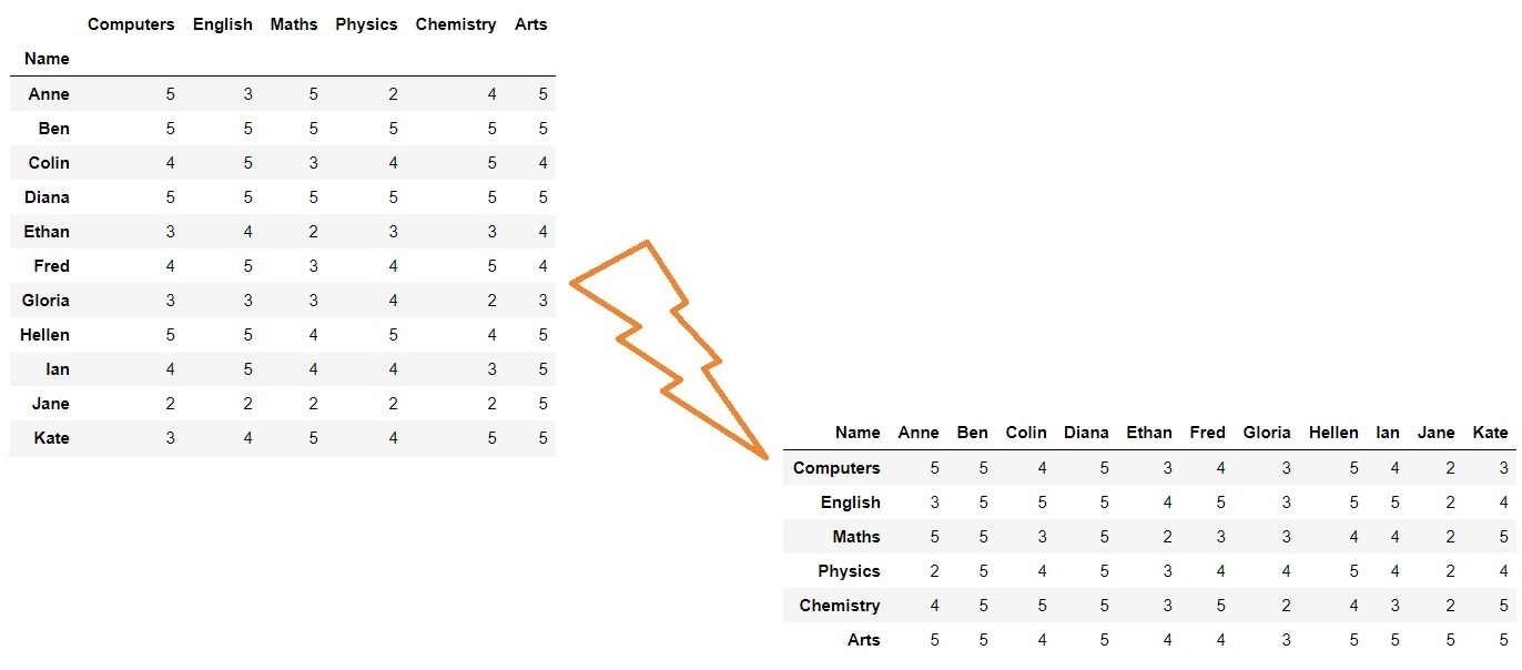
In the table below we have collected the marks of students we have already met in some subjects (Computers, English, Maths, Physics, Chemistry and Arts):
marks = [["Anne",    5, 3, 5, 2, 4, 5],
         ["Ben",     5, 5, 5, 5, 5, 5],
         ["Colin",   4, 5, 3, 4, 5, 4],
         ["Diana",   5, 5, 5, 5, 5, 5],
         ["Ethan",   3, 4, 2, 3, 3, 4],
         ["Fred",    4, 5, 3, 4, 5, 4],
         ["Gloria",  3, 3, 3, 4, 2, 3],
         ["Hellen",  5, 5, 4, 5, 4, 5],
         ["Ian",     4, 5, 4, 4, 3, 5],
         ["Jane",    2, 2, 2, 2, 2, 5],
         ["Kate",    3, 4, 5, 4, 5, 5]]
Let's turn this into an indexed DataFrame
marks_df = pd.DataFrame(marks)
marks_df.columns=["Name", "Computers", "English", "Maths", "Physics", "Chemistry", "Arts"]
marks_ix = marks_df.set_index("Name")
marks_ix
Computing the average mark per subject is easy: we just apply mean to each column of the table:
for subj in marks_ix.columns:
    print(subj, "->", round(marks_ix[subj].mean(), 2))
To compute the average mark per student we shall apply mean to the rows of the table, which we access using loc. As a warm-up let us compute the average mark for Kate:
print("Kate's marks:")
print(marks_ix.loc["Kate"])
print("The average mark:", round(marks_ix.loc["Kate"].mean(), 2))
The names of all the students are located in the index column, so the average mark of each student in the table can be computed like this:
for student in marks_ix.index:
    print(student, "->", round(marks_ix.loc[student].mean(), 2))
7.4. Transposing a table
Transposing a table is an operation that swaps the rows and columns of the table so that the first row swaps with first column, the second row swaps with the secong column and so on. When transposing an indexed DataFrame the names of the columns become the index row of the new table, while the index row gives names of the columns in the new table.
Recall that DataFrames are optimized for efficient access to columns of the table. Therefore, it is convenient to transpose a table which has a few very long rows. Of coruse, we don't have to transpose a table to be able to work with it efficiently (since loc gives access to rows of the table), so transposing a table is a matter of taste or convenience.
To transpose a table just apply T to get the new, transposed table. For example recall that:
marks_ix
After transposing:
marks_tr = marks_ix.T
the new table looks line this:
marks_tr
Let's check what happened to index and columns. In the original table we have:
marks_ix.index
marks_ix.columns
while in the transposed table we have:
marks_tr.index
marks_tr.columns
As we have already seen, the average mark per subject can be computed easily:
for subj in marks_ix.columns:
    print(subj, "->", round(marks_ix[subj].mean(), 2))
To compute the average marks for each student, we can use loc to access the rows of the original table, but we can alsoapply the same logic as above, but to the transposed table:
for student in marks_tr.columns:
    print(student, "->", round(marks_tr[student].mean(), 2))
7.5. Exercises
Exercise 1. Look carefully at the code below and then answer the questions that follow:
import pandas as pd
students = [["Anne",    "f", 13, 46, 160],
            ["Ben",     "m", 14, 52, 165],
            ["Colin",   "m", 13, 47, 157],
            ["Diana",   "f", 15, 54, 165],
            ["Ethan",   "m", 15, 56, 163],
            ["Fred",    "m", 13, 45, 159],
            ["Gloria",  "f", 14, 49, 161],
            ["Hellen",  "f", 15, 52, 164],
            ["Ian",     "m", 15, 57, 167],
            ["Jane",    "f", 13, 45, 158],
            ["Kate",    "f", 14, 51, 162]]
students_df = pd.DataFrame(students)
students_df.columns=["Name", "Sex", "Age", "Weight", "Height"]
students_ix=students_df.set_index("Name")

temp_anomalies = pd.read_csv("data/TempAnomalies.csv", header=None)
temp_anomalies_tr = temp_anomalies.T
temp_anomalies_tr.columns = ["Year", "Anomaly"]
- What is the difference between
students_dfandstudents_ix? - What does
students_ix.indexmean? - What is the value of
students_ix.loc["Fred"]? - What is the value of
students_ix.loc["Fred", "Height"]? - What is the value of
students_df.loc["Fred", "Height"]? - What do you think, why did we apply
Ttotemp_anomalies? - How many columns does
temp_anomalies_trhave?
Exercise 2. This is an overview of spendings of a family over a year (in the local currency):
| Item | Jan | Feb | Mar | Apr | May | Jun | Jul | Aug | Sep | Oct | Nov | Dec |
|---|---|---|---|---|---|---|---|---|---|---|---|---|
| Rent | 8,251 | 8,436 | 8,524 | 8,388 | 8,241 | 8,196 | 8,004 | 7,996 | 7,991 | 8,015 | 8,353 | 8,456 |
| Electricity | 4,321 | 4,530 | 4,115 | 3,990 | 3,985 | 3,726 | 3,351 | 3,289 | 3,295 | 3,485 | 3,826 | 3,834 |
| Phone (landline) | 1,425 | 1,538 | 1,623 | 1,489 | 1,521 | 1,485 | 1,491 | 1,399 | 1,467 | 1,531 | 1,410 | 1,385 |
| Phone (cell) | 2,181 | 2,235 | 2,073 | 1,951 | 1,989 | 1,945 | 3,017 | 2,638 | 2,171 | 1,831 | 1,926 | 1,833 |
| TV and Internet | 2,399 | 2,399 | 2,399 | 2,399 | 2,399 | 2,399 | 2,399 | 2,399 | 2,399 | 2,399 | 2,399 | 2,399 |
| Transport | 1,830 | 1,830 | 1,830 | 1,830 | 1,950 | 1,950 | 1,450 | 1,450 | 1,950 | 1,950 | 2,050 | 2,050 |
| Food | 23,250 | 23,780 | 24,019 | 24,117 | 24,389 | 24,571 | 24,736 | 24,951 | 25,111 | 25,389 | 25,531 | 25,923 |
| Rest | 4,500 | 3,700 | 5,100 | 3,500 | 2,750 | 4,250 | 7,320 | 8,250 | 3,270 | 4,290 | 3,200 | 8,390 |
This table represented as a list looks like this:
spendings = [
  ["Rent", 8251, 8436, 8524, 8388, 8241, 8196, 8004, 7996, 7991, 8015, 8353, 8456],
  ["Electricity", 4321, 4530, 4115, 3990, 3985, 3726, 3351, 3289, 3295, 3485, 3826, 3834],
  ["Landline", 1425, 1538, 1623, 1489, 1521, 1485, 1491, 1399, 1467, 1531, 1410, 1385],
  ["Cell", 2181, 2235, 2073, 1951, 1989, 1945, 3017, 2638, 2171, 1831, 1926, 1833],
  ["TV and Internet", 2399, 2399, 2399, 2399, 2399, 2399, 2399, 2399, 2399, 2399, 2399, 2399 ],
  ["Transport", 1830, 1830, 1830, 1830, 1950, 1950, 1450, 1450, 1950, 1950, 2050, 2050],
  ["Food", 23250, 23780, 24019, 24117, 24389, 24571, 24736, 24951, 25111, 25389, 25531, 25923],
  ["Rest", 4500, 3700, 5100, 3500, 2750, 4250, 7320, 8250, 3270, 4290, 3200, 8390]
]
(a) Convert this list into a DataFrame and index it.
(b) Calculate the average spending of this family per item (Rent, Electricity etc).
Exercise 3. Five groups of students took part in a student poll about their favourite movie genres. Each student was allowed to vote for exactly one genre. The results of the poll are summarized below:
| Genre | Group 1 | Group 2 | Group 3 | Group 4 | Group 5 |
|---|---|---|---|---|---|
| Comedy | 4 | 3 | 5 | 2 | 3 |
| Horror | 1 | 0 | 2 | 1 | 6 |
| SF | 10 | 7 | 9 | 8 | 9 |
| Adventure | 4 | 3 | 4 | 2 | 2 |
| History | 1 | 0 | 2 | 0 | 0 |
| Romance | 11 | 10 | 7 | 9 | 8 |
(a) COnvert this into a DataFrame indexed by genre.
(b) Compute the number of votes per genre.
(c) For each group compute the total number of students that took part in polling.
(d) What is the total number of students that took part in polling?
Exercise 4. Nutritive data for certain products in given in the table below:
| Product (100g) | Nutritive value (kcal) | Carbohydrates (g) | Proteins (g) | Fats (g) |
|---|---|---|---|---|
| Rye bread | 250 | 48.2 | 8.4 | 1.0 |
| White bread | 280 | 57.5 | 6.8 | 0.5 |
| Cheese spread | 127 | 4.0 | 3.1 | 10.5 |
| Margarin | 532 | 4.6 | 3.2 | 1.5 |
| Yoghurt | 48 | 4.7 | 4.0 | 3.3 |
| Milk (2.8%) | 57 | 4.7 | 3.3 | 2.8 |
| Salami | 523 | 1.0 | 17.0 | 47.0 |
| Ham | 268 | 0.0 | 25.5 | 18.4 |
| Chicken breast | 110 | 0.0 | 23.1 | 1.2 |
In the cell below we have converted this table into a DataFrame indexed by the product name:
food = pd.DataFrame([
    ["R-bread", 250, 48.2, 8.4, 1.0],
    ["W-bread", 280, 57.5, 6.8, 0.5],
    ["Spread", 127, 4.0, 3.1, 10.5],
    ["Margarin", 532, 4.6, 3.2, 1.5],
    ["Yoghurt", 48, 4.7, 4.0, 3.3],
    ["Milk", 57, 4.7, 3.3, 2.8],
    ["Salami", 523, 1.0, 17.0, 47.0],
    ["Ham", 268, 0.0, 25.5, 18.4],
    ["ChBreast", 110, 0.0, 23.1, 1.2]])
food.columns=["Product", "NutrVal", "Carbs", "Proteins", "Fats"]
food_ix = food.set_index("Product")
(a) For his breakfast Mike had two pieces of white bread and had a cup of milk. Each piece of bread had some cheese spread and a slice of ham. What is the nutritive value of Mike's breakfast (in kcal) if we assume that each piece of bread weighs 100g, that 10h of spread was used per piece of bread, that one slice of ham weighs 20g and that a cup of milk contains 200 d of milk?
(b) How much fat was there in Mike's breakfast?
(c) Visualize the amount of carohydrates in these products.
Exercise 5. The temperature anomaly is a number that tells us how much the average temperature in a particular year deviates from the optimal value. The file TempAnomalies.csv located in the folder data contains the temperature anomalies (in degrees Celsius) for the peroid of 40 years (1977-2017). The file has two rows like this:
1977,1978,1979,1980,1981,...
0.22,0.14,0.15,0.3,0.37,...
(a) Load the table into a DataFrame (Note: the table has no header so you need the header=None option in your read_scv.)
(b) Transpose the table and call the two columns "Year" and "Anomaly".
(c) Index the table.
(d) Visualize the temperature anomalies by a line chart.
